
FX attribution exercise#
What do we mean by FX attribution?#
The objective of performance attribution, as stated by Menchero (2000) [Men00], is to:
A. Explain portfolio performance relative to a benchmark.
B. Identify the sources of excess return.
C. Relate them to active decisions by the portfolio manager.
In this Jupyter Book we will try to deepen our understanding of B) the sources of excess return in a portfolio. In the case of FX or multicurrency attribution, we are trying to isolate the impact of currency fluctuations on the performance of a portfolio.
For simplicity, in the course of this simple exercise we will not consider excess return, but rather the performance of a portfolio of stocks denominated in two different currencies. This needs to be extended to include the benchmark, which is usually a market index.
Some references for you to explore#
Risk-Adjusted Attribution Campisi (2000) [Cam00] listed the characteristics of a good performance attribution system as follows:
It is consistent with the investment process and the manager’s decision- making process.
It uses a benchmark that reflects the manager’s strategic (long-term) asset allocation.
It measures the effect of the manager’s tactical (short-term) allocation shifts.
It adjusts attribution of return for systematic risk(s).
Rather satisfactorily, Fisher and D’Alessandro (2019) [FDAlessandro19] took attribution full circle and tied risk-adjusted attribution back to the original “Components of Investment Performance” (Fama, 1972 [Fam72]).
See Bacon (2019) [Bac19] for a nice literature review of performance attribution (including multiperiod and multicurrency).
With no further ado, let’s get started!
Portfolio returns breakdown: FX vs stock performance#
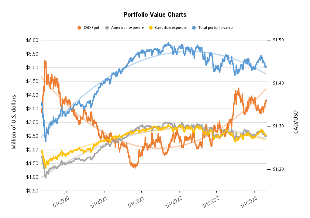
We want to understand the impact of the FX exposure on the portfolio dynamics. We invest in both American and Canadian stocks, so we are exposed to variations in the CADUSD pair. The figure above shows the total dollar value of the portfolio, as well as the breakdown of the Canadian and American exposures.
To run an FX attribution analysis, we will examine the effects of both currency fluctuations and the performance of the stocks in the portfolio.
The Canadian dollar’s appreciation has a direct impact on the value of the Canadian exposure of the portfolio. As the CAD strengthens against the USD, the value of the Canadian stocks held in the portfolio increases when measured in USD. This is because the investor’s holdings in Canadian stocks now have a higher value in U.S. dollars due to the stronger Canadian dollar. On the other hand, the American exposure in the portfolio should remain unaffected by the fluctuations in the CAD/USD exchange rate, as the value of the American stocks is already measured in U.S. dollars.
To understand our FX exposure, we can break down portfolio returns into two components:
Pure FX effect: This represents the change in value of the Canadian exposure due solely to the appreciation of the CAD against the USD. This can be calculated by isolating the change in the CAD/USD exchange rate from the change in the value of the Canadian stocks.
Stock performance effect: This represents the change in the value of the Canadian and American exposure due to the performance of the stocks themselves, independent of the exchange rate fluctuations (recall our discussion on stock valuations, dividend yields, etc.).
By separating the pure FX effect and the stock performance effect, we can identify the contribution of each factor to the portfolio’s overall performance and provide insights for future investment decisions.
Breakdown computation#
Start by calculating the pure FX effect, which measures the impact of changes in exchange rates on the total return of the portfolio. To calculate the pure FX effect for the Canadian portfolio, we use the formula:
Similarly, for the American portfolio:
Next, we calculate the pure stock effect for the American and Canadian portfolios, which measures the impact of changes in stock prices on the total return of the portfolio. We use the formula:
where P is the price of the stock. We calculate this for both American and Canadian exposure. Note that we could expand one step further and consider what we talked about (dividend yield, etc.) as follows:
where \(P^*_t\) is the ex-dividend stock price at time \(t\), \(P_{t-1}\) is the stock price at the previous time period, and \(D_t\) is the dividend payment at time \(t\).
To calculate the total stock effect, we simply add the American and Canadian stock effects together:
To calculate the total FX effect, we use the formulas for the Canadian and American pure FX effect calculated earlier:
Finally, we calculate the total return using the formulas for the total stock effect and total FX effect:
Show code cell source
import requests
import pandas as pd
import matplotlib.pyplot as plt
import seaborn as sns
from matplotlib.ticker import FuncFormatter
import matplotlib.dates as mdates
from matplotlib.ticker import MaxNLocator

# Replace this with your Google Sheets API key
api_key = "AIzaSyAid6kntl2_8pPpYnDQvG1CmrH8fDQwxsg"

# Replace this with your Google Sheet ID
sheet_id = "1NrXdbrLjCDz6pI4o-9xstZ5sS3k_JMALS8ts7dXlBCw"

# Replace this with the name of the sheet/tab you want to access
sheet_name = "Charts"

# Access the Google Sheet
url = f"https://sheets.googleapis.com/v4/spreadsheets/{sheet_id}/values/{sheet_name}!A6:K?key={api_key}"
response = requests.get(url)
result = response.json()
data = result["values"]

# Remove the empty cells from headers
headers = data.pop(0)

df = pd.DataFrame(data, columns=headers)

numeric_columns = [
    "CADUSD",
    "CAD Spot ",
    "Total portfolio value (USD)",
    "Total portfolio value (CAD)",
    "American exposure (USD)",
    "Canadian exposure (USD)",
    "EVOLUTION OF IMPLIED AMERICAN WEIGHT",
    "Return of CAD/USD",
    "American returns",
    "Canadian returns"
]

for col in numeric_columns:
    df[col] = pd.to_numeric(df[col].str.replace('[\$,]', '', regex=True), errors="coerce")
Show code cell source
# Calculate the pure FX effect for the Canadian portfolio
df["Canadian Pure FX Effect"] = ((df["Canadian exposure (USD)"] / df["CADUSD"].shift(1) - df["Canadian exposure (USD)"].shift(1) / df["CADUSD"].shift(1)) * df["CADUSD"])/df["Total portfolio value (USD)"]

# Calculate the pure FX effect for the American portfolio
df["American Pure FX Effect"] = ((df["American exposure (USD)"] * df["CADUSD"].shift(1) - df["American exposure (USD)"].shift(1) * df["CADUSD"].shift(1)) * df["CADUSD"])/df["Total portfolio value (USD)"]

# Calculate the pure stock effect for American exposure
df["American Stock Effect"] = df["American exposure (USD)"].pct_change()

# Calculate the pure stock effect for Canadian exposure
df["Canadian Stock Effect"] = df["Canadian exposure (USD)"].pct_change()

# Calculate the total stock effect
df["Total Stock Effect"] =df["American Stock Effect"] + df["Canadian Stock Effect"]

# Calculate the total FX effect
df["Total FX Effect"] = df["Canadian Pure FX Effect"] + df["American Pure FX Effect"]

# Calculate the total return
df["Total Return"] = df["Total Stock Effect"] + df["Total FX Effect"]

# Set the date column as the index
df.set_index("Date", inplace=True)
Show code cell source
# Set plotting style to scientific
plt.style.use("science")

# Enable LaTeX formatting
plt.rc("text", usetex=True)
plt.rc("font", family="serif")
# Bigger font size in titles and axis labels
plt.rc("axes", titlesize=30)
plt.rc("axes", labelsize=18)
# Bigger font size in legends
plt.rc("legend", fontsize=16)
# Bigger font size in ticks
plt.rc("xtick", labelsize=16)
plt.rc("ytick", labelsize=16)
# Bold font weight in titles and axis labels
plt.rc("axes", titleweight="bold")
plt.rc("axes", labelweight="bold")
# Bold font weight in legends
plt.rc("legend", title_fontsize=16)
plt.rc("legend", labelspacing=0.25)
# Color black for text
plt.rc("text", color="black")

# Function to format y axis as a percentage
def percentage_formatter(x, pos):
    return f"{100 * x:.1f}\%"

# Function to format dates
def format_date(x, pos=None):
    return mdates.num2date(x).strftime("%b-%y")

######################################################################################################
# 1. A line plot showing the evolution of CADUSD, American exposure, and Canadian exposure over time.#
######################################################################################################

# Resample the data to weekly frequency
df["Date"] = pd.to_datetime(df.index)
df.set_index("Date", inplace=True)
weekly_df = df.resample("W").mean()

fig, ax1 = plt.subplots(figsize=(18, 12))

#Line type dashed for CADUSD
ax1.plot(weekly_df.index, weekly_df["CADUSD"], label="CADUSD", color="blue", linestyle="--", linewidth=2, alpha=0.85)
ax1.set_xlabel("Date")
ax1.set_ylabel("CADUSD")
ax1.legend(loc="upper left")

ax2 = ax1.twinx()
ax2.plot(weekly_df.index, weekly_df["American exposure (USD)"], label="American exposure (USD)", color="green", alpha=0.95, linewidth=2)
ax2.plot(weekly_df.index, weekly_df["Canadian exposure (USD)"], label="Canadian exposure (USD)", color="red", alpha=0.95, linewidth=2)
ax2.set_ylabel("Exposure (USD)")
ax2.legend(loc="upper right")

ax1.xaxis.set_major_formatter(FuncFormatter(format_date))
plt.title("CADUSD and Exposure Over Time (Weekly)")
plt.show()
An example of the importance of understanding FX exposure: post-Covid CAD appreciation episode#
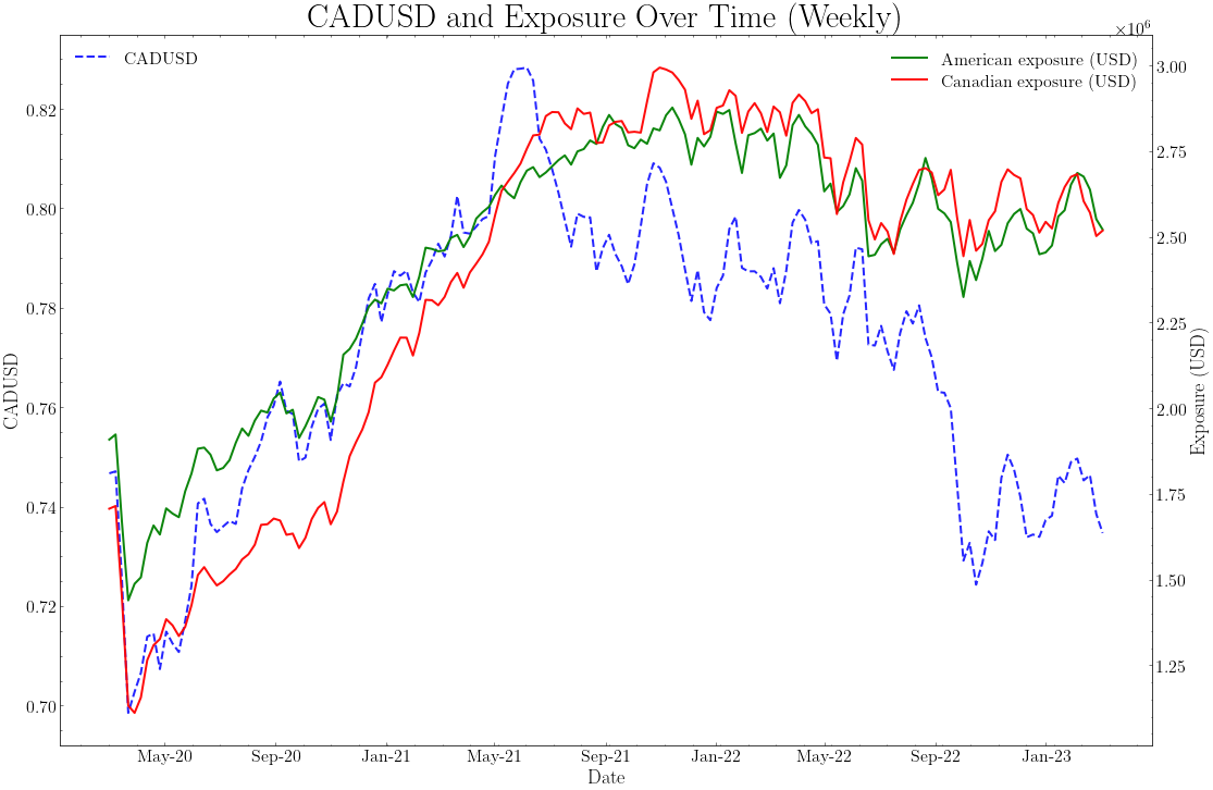
We would expect a stronger performance from the Canadian stocks during a period of CAD appreciation, as the value of the Canadian stocks increases when measured in USD. We can see that this is indeed the case, as the Canadian stocks outperformed the American stocks during the period of CAD appreciation between Feb 2020 and June 2021-i.e., the Canadian exposure grew faster than the American exposure during this period.
Show code cell source
# Max 3 decimal places
pd.options.display.float_format = "{:.3f}".format
df[["American returns", "Canadian returns", "Canadian Pure FX Effect", "American Pure FX Effect", "Total Stock Effect", "Total FX Effect", "Total Return"]].describe()
| American returns | Canadian returns | Canadian Pure FX Effect | American Pure FX Effect | Total Stock Effect | Total FX Effect | Total Return | |
|---|---|---|---|---|---|---|---|
| count | 783.000 | 783.000 | 782.000 | 782.000 | 782.000 | 782.000 | 782.000 |
| mean | 0.000 | 0.001 | 0.000 | 0.000 | 0.001 | 0.000 | 0.001 |
| std | 0.018 | 0.018 | 0.008 | 0.005 | 0.033 | 0.013 | 0.045 |
| min | -0.120 | -0.140 | -0.070 | -0.038 | -0.226 | -0.092 | -0.318 |
| 25% | -0.010 | -0.010 | -0.003 | -0.002 | -0.013 | -0.005 | -0.017 |
| 50% | 0.000 | 0.000 | 0.001 | 0.000 | 0.003 | 0.001 | 0.003 |
| 75% | 0.010 | 0.010 | 0.004 | 0.003 | 0.017 | 0.007 | 0.023 |
| max | 0.110 | 0.110 | 0.042 | 0.027 | 0.183 | 0.056 | 0.239 |
Distribution of FX effects#
Overall, the distributions of American and Canadian returns look fairly similar. This is related with our discussion on CIP deviations. Suppose that the Canadian stocks were on average much more rewarding than the American stocks. Then, we could borrow in USD and invest in Canadian stocks in eternum and arbitrage the difference away. This would lead to a convergence of the two distributions-at least in the long run, for the first moment.
Interestingly, the distributions of the Canadian and American pure FX effects look different. For instance, Canadian Pure FX effect is more volatile than the American. I do not want to spoil the surprise, so I will leave it to you to think about why this is the case and we will discuss it in the next meeting.
Show code cell source
#Plot Total Return
fig, ax = plt.subplots(figsize=(18, 12))
ax.plot(df.index, df["Total Return"], label="Total Return", color="blue", alpha=0.95, linewidth=2)
ax.set_xlabel("Date")
ax.set_ylabel("Total Return")
ax.plot(df.index, df["Total FX Effect"], label="Total FX Effect", color="red", alpha=0.95, linewidth=2)
# Legend
ax.legend(loc="upper right")
ax.xaxis.set_major_formatter(FuncFormatter(format_date))
plt.title("Total Return Over Time")
plt.show()
FX has a “second order” effect on portfolio returns#
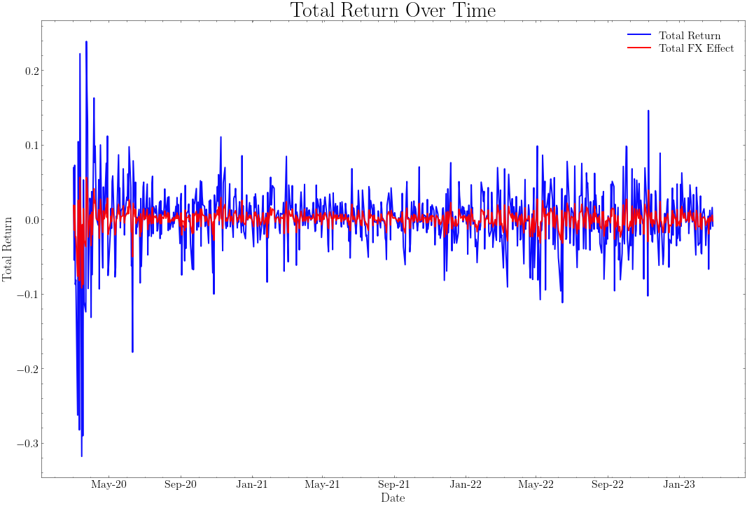
An stylized fact we can take from the figure above is that, in the overall portfolio, the stock performance effect is much more important than the FX effect. This is not surprising. Why? I will leave it to you to think about it and we will discuss it in the next meeting.
Show code cell source
#Plot Cumulative return of the portfolio broken down by stock and FX effects
fig, ax = plt.subplots(figsize=(18, 12))
ax.plot(df.index, (df["Total Stock Effect"] + 1).cumprod(), label="Total Stock Effect", color="blue", alpha=0.95, linewidth=2)
ax.plot(df.index, (df["Total FX Effect"] + 1).cumprod(), label="Total FX Effect", color="red", alpha=0.95, linewidth=2)
#Total return in green and thicker line
ax.plot(df.index, (df["Total Return"] + 1).cumprod(), label="Total Return", color="green", alpha=0.95, linewidth=3)
ax.set_xlabel("Date")
ax.set_ylabel(r"\%")
ax.xaxis.set_major_formatter(FuncFormatter(format_date))
# Add a shadow between Feb 2020 and June 2021 with legend label "U.S. aggressive fiscal response to Covid weakened the USD"
ax.axvspan("2020-02-01", "2021-06-01", alpha=0.2, color="green", label="U.S. aggressive fiscal response to Covid weakened the USD")
#Legend
ax.legend(loc="lower right")
# Add reference of 1.0 on the y axis
ax.axhline(y=1.0, color="black", linestyle="--", linewidth=1)
plt.title(r"Cumulative Returns Breakdown")
plt.show()
More on the CAD appreciation episode#
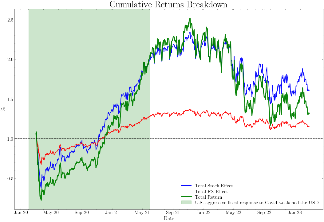
Note how during the aggressive fiscal response to Covid from the Federal Reserve in the U.S. pushed the dollar down and we had a Canadian dollar appreciation. This is a good example of how the FX effect can be important in the overall portfolio performance. However, the stock performance effect was much more important. We should think about an argument to explain why is it worth it to pay attention to this ‘’second order’’ effect. I will leave it to you to think about it and we will discuss it in the next meeting.
Show code cell source
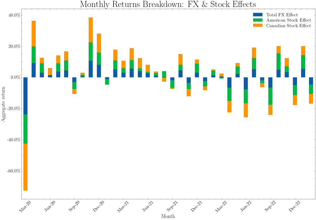
# Aggregate returns by month
returns_decomposition = df[["Total FX Effect", "American Stock Effect", "Canadian Stock Effect"]].dropna()
returns_decomposition = returns_decomposition.resample("M").apply(lambda x: (1+x).prod() - 1)

# Add a "Date" column equal to the index
returns_decomposition["Date"] = returns_decomposition.index

fig, ax = plt.subplots(figsize=(18, 12))
returns_decomposition.plot(x="Date", y=["Total FX Effect", "American Stock Effect", "Canadian Stock Effect"], kind="bar", stacked=True, ax=ax)
ax.set_xlabel(r"Month")
ax.set_ylabel(r"Aggregate return")
ax.yaxis.set_major_formatter(FuncFormatter(percentage_formatter))
ax.set_xticklabels(returns_decomposition["Date"].dt.strftime("%b-%y"), rotation=45)
#Maxmium number of ticks on the x axis is 12
ax.xaxis.set_major_locator(MaxNLocator(12))

plt.title(r"Monthly Returns Breakdown: FX \& Stock Effects")
plt.show()
Pushing the analysis further#
The above is merely a representation of what I have in mind to complete the FX attribution exercise. The numbers are not correct, as I am aggregating returns at the monthly level using daily returns and applying a geometric average without considering an extra drift correction. Try to replicate the above exercise more precisely and:
Breakdown the FX effect into the part that is spanned by the American and Canadian portfolios.
Once you have 1), try to break down the exposure by sectors.
Think about how to incorporate the benchmark to this exercise. This is critical. When it comes to attribution, we need to be able to compare the performance of the portfolio with the performance of the benchmark and express everything in terms of excess returns.