Hedging Your Bets: A Deep Dive into the Asset Pricing Model of Koijen and Yogo

Hedging Your Bets: A Deep Dive into the Asset Pricing Model of Koijen and Yogo#

By Martin Rinaldi and Spencer Dean#

Submitted to: Prof. Alberto Mokak Teguia#

Part I#

The Demand System in Action: A Case Study#

The demand system asset pricing approach is a method to estimate asset prices based on a model of investors’ demand for assets. In this approach, the weight of investor i in stock n at time t is given by the equation:

\[ w_{i,t}(n)=\frac{\delta_{i,t}(n)}{1+\sum_m \delta_{i,t}(m)}, \]

where $\delta_{i,t}(n)$ is a measure of investor i’s demand for stock n at time t, and is defined by the equation:

\[ \delta_{i,t}(n)=\exp\left(\beta_{0,i,t}me_{t}(n) +\beta_{1,i,t}'x_t(n)\right)\epsilon_{i,t}(n), \]

Here, $me_t(n)$ denotes the log market capitalization of stock $n$, $x_t(n)$ denotes the stock’s characteristics, and $ε_{i,t}(n)$ denotes a latent demand factor.

To estimate the model, we need to use instrumental variables (IV) to address endogeneity issues. Two IV estimators are considered in this model. The first is a linear IV estimator, which is implemented by assuming that $E[\ln ε_{i,t}(n)|\widehat{me}_t(n), x_t(n)] = 0$, where $ \widehat{me}_t(n)$ is the instrument. The second estimator is a nonlinear IV estimator, which is implemented by using a simulated method of moments approach.

A sufficient condition for a unique equilibrium in this model is that $β_{0,i} < 0$ for all investors. This condition is imposed in the estimation.

Summary: Demand System Asset Pricing Model

Investor’s demand function: The measure of investor i’s demand for stock n at time t is a function of the log market capitalization, stock characteristics, and a latent demand factor. This latent factor captures unobserved factors affecting investor demand, such as sentiment or macroeconomic conditions.
Model estimation components: Key components include log market capitalization, stock characteristics, and the latent demand factor. The model requires a method to address the endogeneity issue caused by the unobservable latent demand factor.
Instrumental variables (IV) estimation: The model employs two IV estimation techniques to address the endogeneity issue: linear IV estimator and nonlinear IV estimator. The linear IV estimator assumes that the error term is uncorrelated with the instrument and stock characteristics, while the nonlinear IV estimator uses a simulated method of moments approach.
Unique equilibrium: A unique equilibrium is ensured by imposing the sufficient condition that $\beta_{0,i}<0$ for all investors. This prevents multiple equilibria that could arise from conflicting preferences regarding market capitalization.
Replication code: The paper by Ralph S.J. Koijen and Motohiro Yogo provides a replication code for estimating the demand system asset pricing model using data from two prominent institutional investors, Dimensional Fund Advisors and Vanguard, during a specified time period.

Characterization of the IV estimators#

I. Linear#

We first consider a linear IV estimator. If we drop the zero positions, the model implies (with $w_{i,t}(0)$ the fraction invested in the outside asset)

\[ \ln \left(\frac{w_{i,t}(n)}{w_{i,t}(0)} \right) = \beta_{0,i,t}me_{t}(n) +\beta_{1,i,t}'x_t(n)+c_{i,t} + \ln \epsilon_{i,t}(n), \]

and we assume that $\mathbb{E}\left[ \ln \epsilon_{i,t}(n) \mid \widehat{me}_{t}(n),x_t(n) \right] = 0$, with $\widehat{me}_{t}(n)$ the instrument. This is a standard linear IV estimator that is implemented below.

As shows in KY19, a sufficient condition for a unique equilibrium is that $\beta_{0,i}<0$, for all investors. We impose this restriction in the estimation.

II. Non linear#

Next, we also consider a non-linear estimator that uses the moment condition $$ \mathbb{E}\left[\epsilon_{i,t(n)}\mid \widehat{me}_{t}(n),x_t(n) \right] = 1. $$ The advantage of this estimator is that we do not need to drop the zero holdings.

We form the moment conditions: $$ \mathbb{E}\left[\left(\frac{w_{i,t}(n)}{w_{i,t}(0)} \exp\left(-\beta_{0,i,t}me_{t}(n) -\beta_{1,i,t}'x_t(n)\right) - 1\right)\left(\widehat{me}_{t}(n),x_t(n)\right) \right] = 1. $$

To solve the moment conditions, we linearize the moment conditions and use it form an iterative algorithm as in Koijen, Richmond, and Yogo (2020), see https://papers.ssrn.com/sol3/papers.cfm?abstract_id=3378340.

Koijen and Yogo (2019) mainly study two central objects of interest in asset pricing:#

The distribution of price elasticities with respect to demand shocks (residual demand).
Predictability - a central theme in asset pricing.

With respect to the second object, traditionally, return predictability in stock portfolios has been attributed to risk exposure. KY19 propose an alternative explanation, highlighting the importance of investor demand even if unrelated to cash flow expectations or hedging motives

In this notebook, we will focus on the first object of interest, the distribution of price elasticities with respect to demand shocks. Below we modify our original exercise by:

Introducing heterogeneity in the cross-section of institutional investors. Instead of considering only two investors, we consider more than 3000.
Allowing for time variation in the demand parameters. In this exercise, we will consider only two quarters of data as opposed to the static model in the original exercise.

import numpy as np
import pandas as pd
from IPython.display import display, Markdown
import matplotlib.pyplot as plt
import seaborn as sns
sns.set_style('whitegrid')
sns.set_palette('colorblind')
import statsmodels.api as sm
import os, requests, zipfile, io
import ipywidgets as widgets
from IPython.display import display
from joblib import Parallel, delayed
from tqdm import tqdm
from scipy.stats import lognorm
from scipy.interpolate import interp1d
import matplotlib as mpl
mpl.style.use('/Users/martinrinaldi/Dropbox/PhD in Finance/2022-2023/Term 2/Theoretical AP/LucasBonsai/rinaldiplots.mplstyle')

# Read the feather file
df = pd.read_feather('/Users/martinrinaldi/Dropbox/PhD in Finance/2022-2023/Term 2/Theoretical AP/LucasBonsai/data.feather')
# Drop nans and duplicates  
df = df.dropna().drop_duplicates()
# Drop the rows where the variable 'aum' is zero or mgrno is zero
df = df[(df['aum'] != 0) & (df['mgrno'] != 0)]
df = df[['mgrno', 'permno', 'rweight', 'profit', 'Gat', 'divA_be', 'beta', 'LNbe', 'LNme', 'IVme', 'aum']]

from IPython.display import display, HTML

# Number of unique managers
n_mgr = df['mgrno'].nunique()

# Number of unique time periods|
n_time = df['permno'].nunique()

# Summary of statistics
summary = df.describe().round(2).T

summary_table = summary.to_html()

unique_info = f"Number of unique institutions: {n_mgr}"

display(HTML(f"{unique_info}<br><br>{summary_table}"))

Number of unique institutions: 2942

	count	mean	std	min	25%	50%	75%	max
mgrno	987572.0	37292.66	28631.62	110.00	10895.00	27800.00	63895.00	95110.00
permno	987572.0	61562.57	27827.03	10001.00	36468.00	76076.00	85728.00	93105.00
rweight	987572.0	0.25	31.40	0.00	0.00	0.00	0.03	21161.24
profit	987572.0	0.25	0.28	-1.82	0.16	0.26	0.37	0.83
Gat	987572.0	0.11	0.20	-0.49	0.01	0.08	0.17	0.85
divA_be	987572.0	0.03	0.04	0.00	0.00	0.02	0.05	0.15
beta	987572.0	1.23	0.69	-0.12	0.71	1.12	1.60	3.86
LNbe	987572.0	7.37	1.99	-5.30	6.02	7.27	8.86	11.91
LNme	987572.0	8.02	2.12	-1.11	6.55	7.97	9.60	13.15
IVme	987572.0	7.96	0.58	1.07	7.62	7.99	8.33	9.30
aum	987572.0	29933.78	82540.18	10.05	438.16	3208.40	17660.10	698625.57

_images/e31776887ce9d234777e197e9e424e59b6466cb52d2e008814565f587dd53069.png

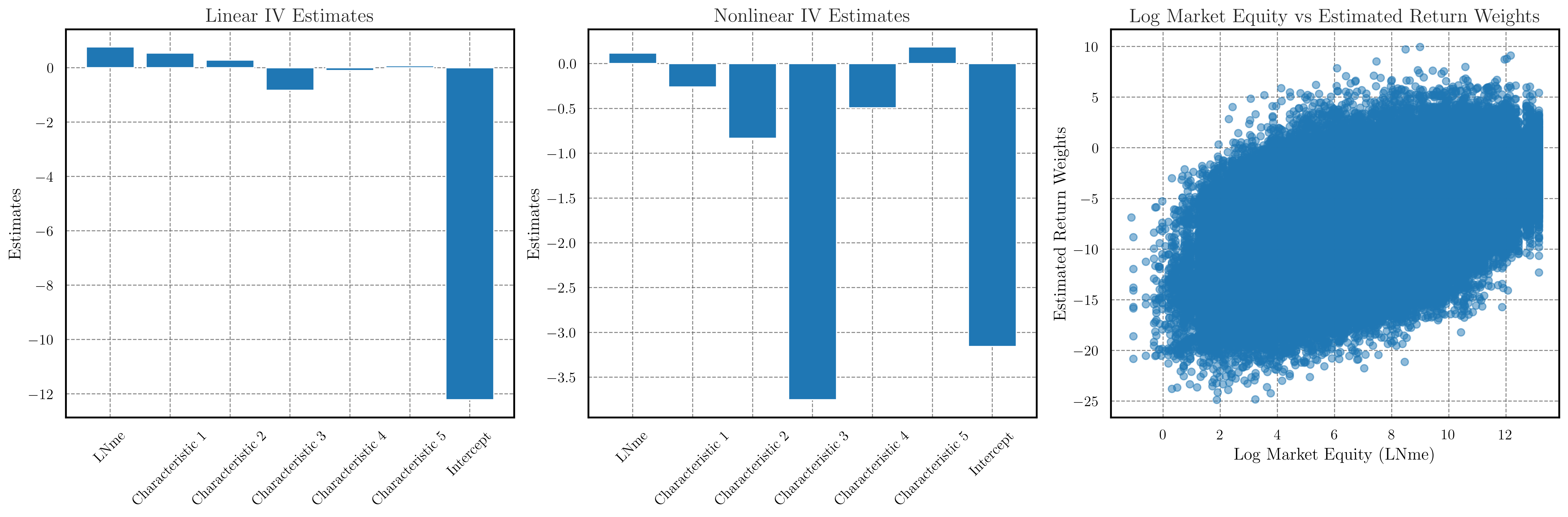
Interpretation of estimates#

Vanguard - Linear IV and Nonlinear IV Estimates#

Linear IV Estimates and Nonlinear IV Estimates are equivalent–i.e., robustness of the linear IV method.

LnME: The coefficient for LnME is 1.0. As the market equity of an asset increases, investors are more likely to allocate a larger portion of their portfolio to that asset.
Note how, differently from our previous result–static, 2 firms case–the coefficients’ estimates are quite different between implementing a linear instrument and a nonlinear. The gap is particularly large for the characteristic 3, which implies that–when allowing for enriched heterogeneity in the cross-section of institutional investors–nonlinearities emerge in the relationship between some characteristics and the demand for assets.
Intercept: The difference in intercepts between the linear and nonlinear instrument cases is striking. Recall that the intercept represents the implied value that investors assign, on average, to the outside option in terms of revealed preference.

Note:

In this context, the positive coefficient for LnME may indicate a departure from the sufficient condition for a unique equilibrium.

Computing price elasticity of demand for a specific security#

To estimate the price elasticity of demand for a specific security with a unique identifier “permno,” we can adapt the model that captures the demand system of a particular investor to handle dynamic estimation. Below we illustrate this method.

def run_analysis(mgrno, permno=None, display_output=True, suppress_print=False):

    # Load data
    mdata = np.array(pd.read_excel('/Users/martinrinaldi/Dropbox/PhD in Finance/2022-2023/Term 2/Theoretical AP/LucasBonsai/DataEstimation.xlsx'))
    mdata = mdata[mdata[:, 0] == mgrno]
    if permno is not None:
        mdata = mdata[mdata[:, 1] == permno]
    if len(mdata) == 0:
        if not suppress_print:
            print("Insufficient data for the selected PERMNO.")
        return
    vrweight = mdata[:, 2:3]

    ###############################
    # Linear IV Estimation ########
    ###############################
    # Identify the nonzero weights
    vloc = np.argwhere(vrweight > 0)[:, 0]

    # Select the data with nonzero weights
    mdata0 = mdata[vloc]
    mchars = mdata0[:, 3:8]
    vLNme = mdata0[:, 8:9]
    vLNmeIV = mdata0[:, 9:10]
    vLNrweight = np.log(vrweight[vloc])

    dT = len(vLNme)
    vones = np.ones((dT, 1))

    # Construct the matrix X and matrix Z
    mX = np.concatenate([vLNme, mchars, vones], axis=1)
    mZ = np.concatenate([vLNmeIV, mchars, vones], axis=1)

    # Check if there are enough data points with nonzero weights
    if len(vloc) < 1:  # You can adjust this threshold to your preference
        if not suppress_print:
            print("Insufficient data with nonzero weights for the selected PERMNO.")
        return

    # Unconstrained linear IV estimation
    vb_linearIV = np.linalg.pinv(mZ.T @ mX) @ mZ.T @ vLNrweight

    # Constrained linear IV estimation
    if vb_linearIV[0] > .99:
        mX = np.concatenate([mchars, vones], axis=1)
        vb_linearIV = np.linalg.inv(mX.T @ mX) @ mX.T @ (vLNrweight - .99 * vLNme)
        vb_linearIV = np.concatenate([np.array([[.99]]), vb_linearIV], axis=0)

    ###############################
    # Non-linear IV Estimation ####
    ###############################

    # Reconstruct the matrix X and matrix Z
    mX = np.concatenate([vLNme, mchars, vones], axis=1)
    mZ = np.concatenate([vLNmeIV, mchars, vones], axis=1)

    # Unconstrained nonlinear IV estimation
    vb_nonlinearIV = vb_linearIV
    dchange = 1

    while dchange > 1e-4:
        vlatent = vrweight[vloc].reshape(-1, 1) * np.exp(-mX @ vb_nonlinearIV)
        mZ_tilde = (vlatent @ np.ones((1, dN))) * mZ

        vb_nonlinearIV_new = vb_nonlinearIV + np.linalg.pinv(mZ_tilde.T @ mX) @ mZ.T @ (vlatent - 1)

        dchange = np.max(np.abs(vb_nonlinearIV - vb_nonlinearIV_new))

        vb_nonlinearIV = vb_nonlinearIV_new

    # Calculate price elasticity
    price_elasticity = -vb_nonlinearIV[0] * (1 / (1 - vb_nonlinearIV[0]))

    if not display_output:
        return price_elasticity, np.mean(mdata0[:, 2])

    if display_output:
        if permno is not None:
            print(f'Estimated Price Elasticity of Demand for PERMNO {permno}: {price_elasticity[0]:.2f}')
        return
    

def on_button_click(button):
    institution = dropdown.value
    permno = permno_input.value
    if permno != "":
        try:
            permno = int(permno)
        except ValueError:
            print("Invalid PERMNO. Please enter a valid integer.")
            return
    else:
        permno = None
    run_analysis(institution, permno)
    
def plot_elasticities(elasticities, market_caps, mgrno):
    plt.figure(figsize=(10, 6))
    
    for i, (label, color) in enumerate(zip(["Vanguard", "DFA"], ["blue", "green"])):
        plt.scatter(market_caps[i], elasticities[i], c=color, label=label)
    
    plt.xscale("log")
    plt.xlabel("Average Market Capitalization")
    plt.ylabel("Price Elasticity of Demand")
    plt.legend()
    plt.title(f"Price Elasticity of Demand vs. Average Market Capitalization for {mgrno}")
    plt.show()

def compute_elasticities(mgrno):
    mdata = np.array(pd.read_excel('/Users/martinrinaldi/Dropbox/PhD in Finance/2022-2023/Term 2/Theoretical AP/LucasBonsai/DataEstimation.xlsx'))
    mdata = mdata[mdata[:, 0] == mgrno]
    unique_permnos = np.unique(mdata[:, 1])

    # Define a helper function for parallel processing
    def process_permno(permno):
        result = run_analysis(mgrno, permno, display_output=False, suppress_print=True)
        if result is not None:
            elasticity, avg_market_cap = result
            return (elasticity, avg_market_cap)
        else:
            return None

    # Run the analysis in parallel with a progress bar
    num_cores = -1  # Use all available cores
    results = Parallel(n_jobs=num_cores)(delayed(process_permno)(permno) for permno in tqdm(unique_permnos, desc="Processing PERMNOs"))

    # Extract elasticities and market_caps from the results
    elasticities = []
    market_caps = []
    for result in results:
        if result is not None:
            elasticity, avg_market_cap = result
            elasticities.append(elasticity)
            market_caps.append(avg_market_cap)

    return elasticities, market_caps


def on_plot_button_click(button):
    mgrno_vanguard = 23001
    mgrno_dfa = 23000
    
    elasticities_vanguard, market_caps_vanguard = compute_elasticities(mgrno_vanguard)
    elasticities_dfa, market_caps_dfa = compute_elasticities(mgrno_dfa)
    
    plot_elasticities([elasticities_vanguard, elasticities_dfa],
                      [market_caps_vanguard, market_caps_dfa],
                      "Vanguard and DFA")

# Create a dropdown widget to choose the institution
dropdown = widgets.Dropdown(
    options=[('DFA', 23000), ('Vanguard', 90457)],
    value=23000,
    description='Institution:'
)

# Create an input widget for the PERMNO
permno_input = widgets.Text(
    placeholder='Enter PERMNO',
    description='PERMNO:',
    disabled=False
)

# Create a button to run the analysis
button = widgets.Button(
    description='Run Analysis',
    button_style='success'
)
button.on_click(on_button_click)

plot_button = widgets.Button(description="Plot Elasticities")
plot_button.on_click(on_plot_button_click)

# Display the widgets
display(dropdown)
display(permno_input)
display(button)
display(plot_button)

Estimated Price Elasticity of Demand for PERMNO 17144: 0.20

Processing PERMNOs: 0it [00:00, ?it/s]
Processing PERMNOs: 100%|██████████| 2776/2776 [03:49<00:00, 12.11it/s]

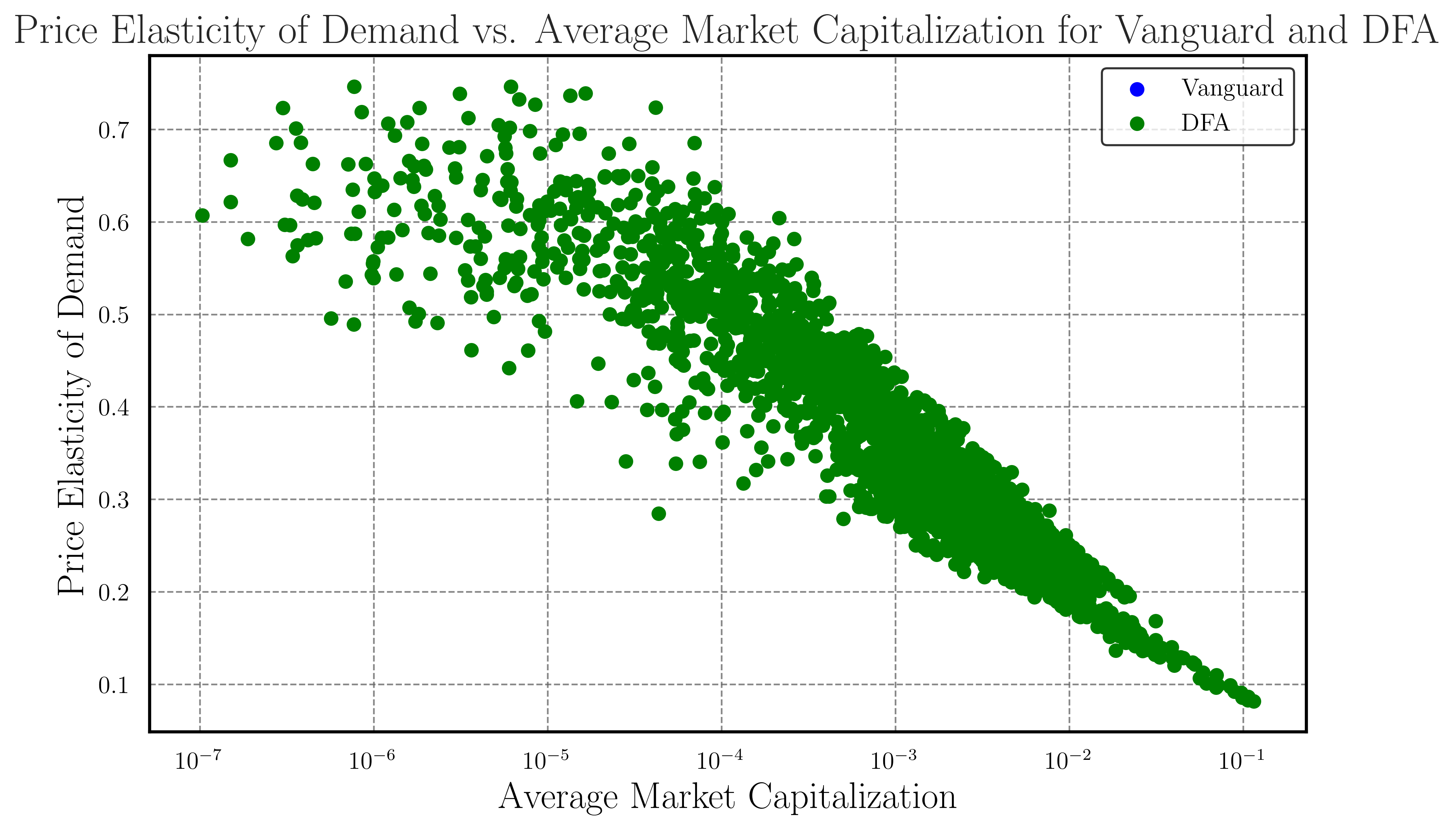
_images/721e13756356b529198256bb4706ba0597155dba205f57107254441bc447165c.png

Demand of these particular investors for stocks with lower market capitalization is more sensitive to changes in prices with respect to larger companies. Suppose we run this exercise for a large set of investors, recover the full demand system, and price elasticity of demand for all available assets within a class. We might be able to breakdown what part of this sensitivity stems from the “latent demand” and idiosyncratic features — fascinating.

# Read data and select manager
mgrno = 23000

mdata = np.array(pd.read_excel('/Users/martinrinaldi/Dropbox/PhD in Finance/2022-2023/Term 2/Theoretical AP/LucasBonsai/DataEstimation.xlsx'))
mdata = mdata[mdata[:, 0] == mgrno]

Processing PERMNOs: 100%|██████████| 2776/2776 [03:59<00:00, 11.61it/s]

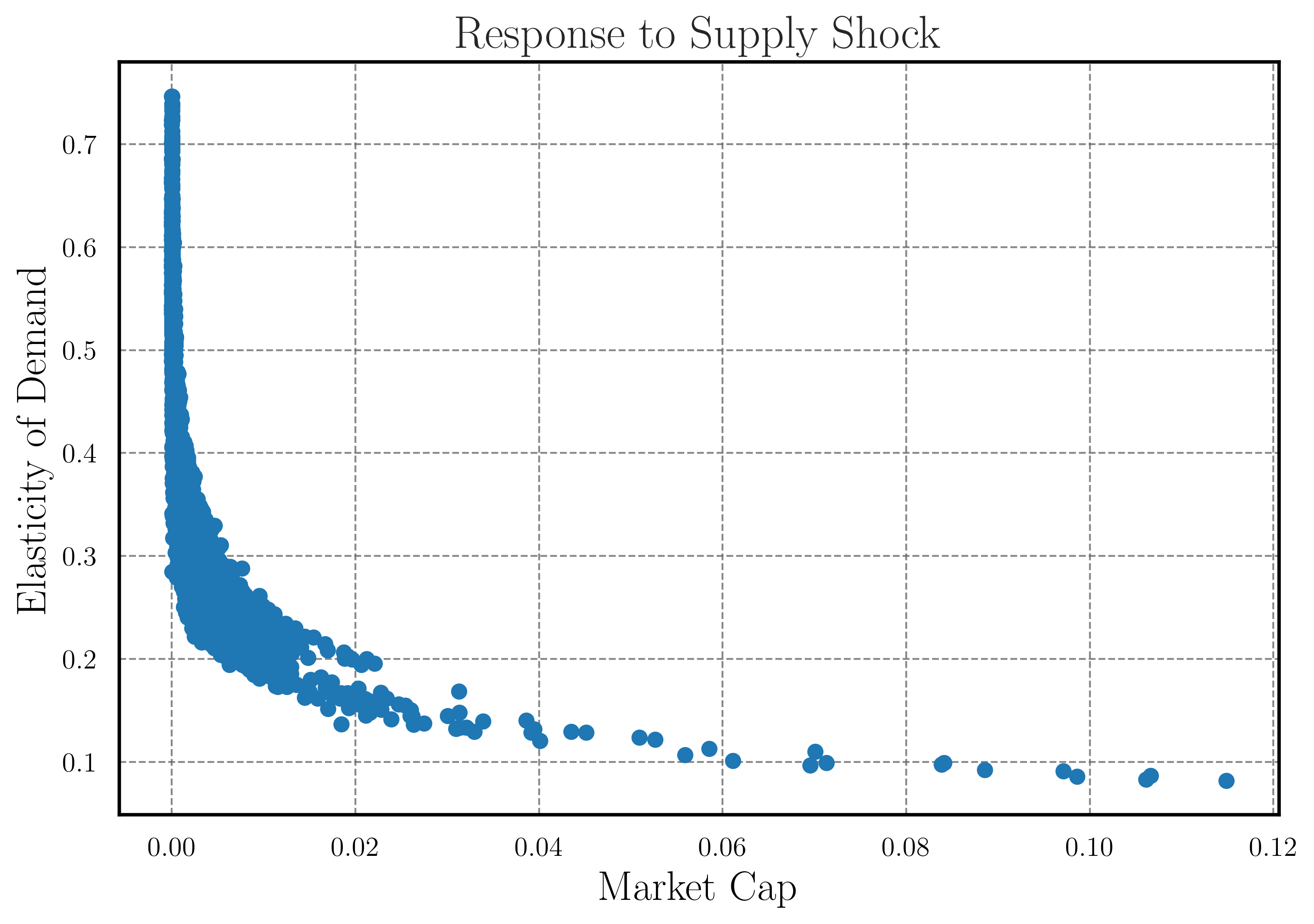
_images/79e665facd1796c3b755995dc14c118257d793367b38dc3448644898bf60c823.png

A 10% negative supply shock in shares outstanding has changed the relationship between market capitalization and elasticity of demand. The hyperbolic shape of the elasticity of demand curve in response to a negative supply shock can be suggestive of many things - e.g., the presence of market frictions, such as illiquidity at low market capitalization levels.

Note: Our analysis of the elasticity of demand in response to a negative supply shock challenges the assumption of fixed supply in the model and highlights the need to consider market frictions and changes in the supply side to better understand the dynamics of asset prices. We want to focus on testing for robustness of KY19 to changes in supply conditions. However, the change is smoother than before. This is due to the fact that the outside option is being ``forced’’ to be the complement of the observed weights. This is entirely an econometric issue that cannot be attributed to the model.

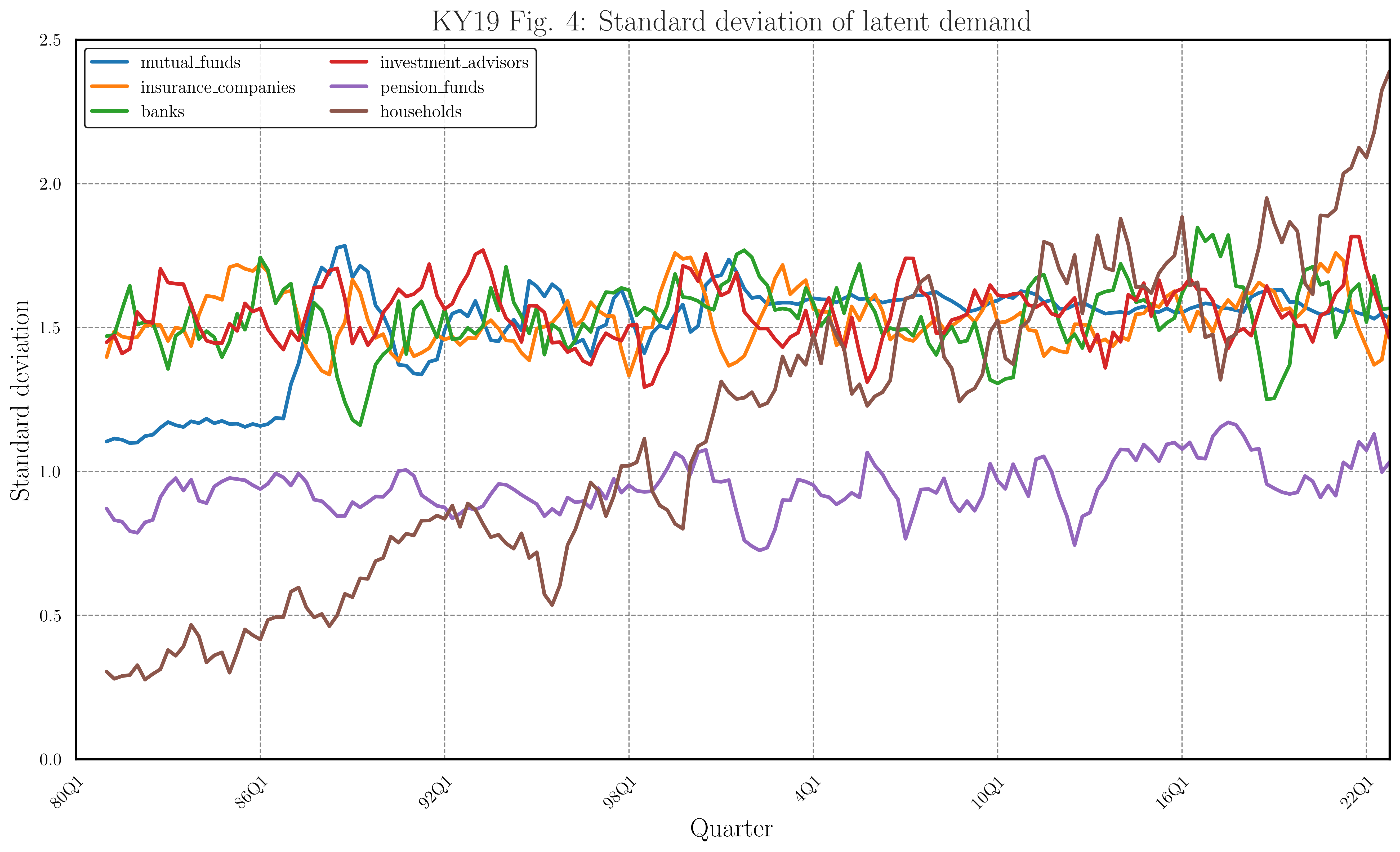
Part II: The unexploited heterogeneity in latent demand#

In this section, we will replicate Figure 4 of KY19. The figure shows the evolution of the latent demand component in the cross-section of investors.

The intention is for this section to motivate the extension that we discuss in the main document.

# Convert 'quarters' column to datetime format
data['quarters'] = pd.to_datetime(data['quarters'])

# Create the figure and set its size
fig, ax = plt.subplots(figsize=(16, 9))

# Plot the time series
for col in data.columns[1:]:
    ax.plot(data['quarters'], data[col], label=col)

# Set y-axis range and label
ax.set_ylim(0, 2.5)
ax.set_ylabel('Standard deviation')

# Set x-axis range, ticks, and label
ax.set_xlim(data['quarters'].iloc[0], data['quarters'].iloc[-1])
n_quarters = len(data)
ax.set_xticks(data['quarters'][::n_quarters // 7])  # Show 8 tick labels maximum

ax.set_xticklabels([f"{q.year % 100}Q{q.quarter}" for q in data['quarters'][::n_quarters // 7]])

# Rotate 45 degrees the x-axis labels
plt.setp(ax.get_xticklabels(), rotation=45, ha="right", rotation_mode="anchor")

ax.set_xlabel('Quarter')
# Add title: KY19 Figure 4: Standard deviation of latent demand
ax.set_title(r'KY19 Fig. 4: Standard deviation of latent demand')
# Add legend small and in a box with a background light color and thick border
ax.legend(loc='upper left', frameon=True, framealpha=0.9, facecolor='white', edgecolor='black', ncol=2)
# Show the figure
plt.show()

_images/967cc621f1fb4fc6ec611ac5cc2d05aad675f58dd36b34dc5d90b84c7ca15b9e.png

REFERENCES#

Koijen, R. S., & Yogo, M. (2019). A demand system approach to asset pricing. Journal of Political Economy, 127(4), 1475-1515.
Koijen, R. S., Richmond, R. J., & Yogo, M. (2020). Which investors matter for equity valuations and expected returns? (No. w27402). National Bureau of Economic Research.